Breaking

Symmetries

Each of the four fundamental forces is characterised by a set of symmetry transformations. A symmetry is a change that you can make under which something remains the same. So, for example, a “reflection” is a transformation, under which left and right are swapped over:

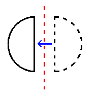
A reflection

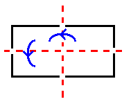
A rectangle has two reflection symmetries:

Another example of a transformation is a rotation. This could, for example, be a rotation in two dimensions. A two-dimensional object can be rotated through any number of degrees: 20º, 59º or even 241.799868º. This kind of transformation is called a continuous symmetry, while a reflection is an example of a discrete symmetry – there is no halfway house between making a transformation and not making one; you can’t “reduce” the “amount” of a reflection.

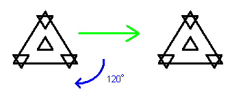
Triangles are symmetric only under rotations which are multiples of 120º:

while circles are symmetric under any rotation in two dimensions.

These symmetry transformations can be combined by carrying out one after another. Combining symmetries in this way allows one to construct “groups” of symmetry transformations. The study of these groups of symmetries is called group theory. Again, there is a host of information available on group theory. If you are wanting to explore group theory for the first time, I’d highly recommend Teach Yourself Mathematical Groups by Tony Barnard and Hugh Neill, in the Hodder & Stoughton Teach Yourself series.

Rotations can obviously be defined in three dimensions as well. A sphere is perfectly symmetric under three-dimensional rotations. Rotations can equally be defined in higher numbers of dimensions. As mentioned on the page “warping”, changes of reference frame in special relativity can be described as rotations in four-dimensional spacetime.

Typically, in fundamental physics, the symmetry will preserve the field equations.

The field equations of general relativity are preserved by changes of the coordinates used on the spacetime. These changes of coordinates induce transformations on the tangent spaces. The symmetries of tangent spaces are much simpler than those of the underlying curved space. If we exclude discrete symmetries such as reflections, they essentially fall into two categories: those which preserve the lengths of lines and the angles between them – i.e. rotations – and those which don’t.

My analysis of these symmetries can be found in the following preprint:

Tangent space symmetries »

Preprint of an article published in International Journal of Geometric Methods in Modern Physics, 2021 https://doi.org/10.1142/S0219887821400089 © World Scientific Publishing Company

Complex numbers

The symmetries characterising the other three interactions are based on a type of number called a complex number. In this subsection, we explain what these are – skip it if you’re already familiar with these. If you’re not, and you want more detail than I’m giving here, a simple internet search should give you a much fuller description of them.

Any number n can be multiplied itself to create its square, n². For example, 3² = 3 x 3 = 9. This is an example of an operation known as a map; it “maps” the number 3 to the number 9. This map can be inverted, to take us from 9 back to 3. This inverse is known as the square root. The square root of any number n is denoted √n or n^½. For example, 9^½ = 3 and 25^½ = 5.

Negative numbers can also be squared, for example (-4)² = -4 x -4 = 16 and (-1)² = -1 x -1 = 1. Positive and negative numbers, such as those in these examples, are called real numbers.

Any positive number has two square roots, both of which are real numbers. One is positive and the other is negative. That is, for any positive number x it is always possible to find a positive number y that has the property y² = x; corresponding to y, there is then a negative number –y which also squares to x: (-y)² = x.

However, the square root of a negative number is not a real number. There is no positive or negative number, for example, which squares to -4. What mathematicians (and physicists) do at this point is to invent a new kind of number, called an imaginary number. They use the letter i to denote the “imaginary” square root of -1, that is, i x i = -1. This number can be multiplied by a real number to create another imaginary number, such as 4i = 4 x i. Any such imaginary number will square to a negative number: (4i)² = 4 x i x 4 x i = 4 x 4 x i x i = 16 x -1 = -16. Conversely, the square root of any negative number is an imaginary number: (-9)^½ = 3i. A real number can then be added to an imaginary number to create a complex number, such as 4 + 3i. Perhaps surprisingly, the normal rules of arithmetic can be extended very simply to cover imaginary numbers.

Now this is all just number theory so far (although certainly interesting in its own right). But it turns out that complex numbers are extremely useful in mathematics and physics. They are very helpful in describing wave motion, for example. And they are also very helpful in describing what physicists call “fermionic matter”: matter-like particles, such as electrons, the quarks which are fundamental components of protons and neutrons, and indeed protons and neutrons themselves.

Internal symmetries

Subatomic particles can often be classified into sets where every member of a set is identical apart from one label – for example, you could have a pair of particles which are identical apart from the fact one has a positive electric charge and the other has a negative electric charge. Thus if the equations governing the motion of a set of charged particles don’t change if positively charged particles are substituted for identical negatively charged ones, and vice versa, those equations can be said to be symmetric under a change of charge.

The symmetry groups underlying the electromagnetic, strong and weak interactions relate to these kinds of particle identities. These groups have a similar structure to groups of rotations. In fact, they can be described as rotations of complex vectors – vectors which are characterised by complex numbers. For example, the strong interaction is based on a symmetry group called SU(3). This group describes rotations of a three-dimensional complex vector, that is, a vector in a three-dimensional space where each of the coordinates is a complex number. (Note that we don’t need to know whether this rather peculiar space has any physical meaning in order to carry out physics calculations. That is certainly an interesting question, but it’s enough to know that the mathematics works to do most particle physics calculations.)

Sometimes, the groups of rotations in complex spaces have exactly the same structure as groups of rotations in real spaces. For example, any rotation in two complex dimensions corresponds to two different rotations in three real dimensions. This correspondence holds when rotations are combined: if we combine two rotations, A and B, in the complex space, we get a complex rotation which corresponds to a rotation C in the real space; combining the rotations corresponding to A and B in the real space results in the same rotation C.

There is a similar correspondence between rotations in a four-dimensional complex space and those in a six-dimensional real space. This is analysed in a paper I co-wrote with Ken Barnes and Jason Hamilton-Charlton:

How orbits of SU(N) can describe rotations in SO(6) »

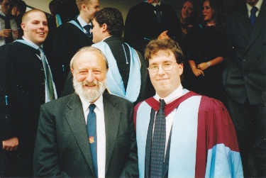
Me with Ken Barnes on the day of my PhD graduation

Unification

The ultimate goal of physicists investigating the four interactions is to develop a single theory which describes all of them and the way they interact with the known fundamental particles. It is unclear what type of theory this would be; it could be a geometric theory, a quantum field theory as most physicists seem to think, or something else completely. (A quantum field theory is a theory which is consistent with both quantum mechanics and special relativity, in which fundamental particles are described as excitations of a field.) However, it’s pretty clear that a key feature of the theory would be its symmetries.

Over the course of the 20th century, there was considerable progress in unifying the forces in this way.

In the 1960s, a theory was proposed by Abdus Salam and Steven Weinberg for unifying the electromagnetic and weak interactions. This theory predicted the existence of a number of new particles, including the famous Higgs particle, which have since been discovered.

Salam and Weinberg’s theory was later extended to incorporate the strong nuclear force, although it turned out there was no unique way to do this.

The “electroweak theory” is based on the concept of symmetry breaking.

Symmetry breaking

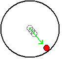
This concept is best described by way of an analogy. Imagine taking a sombrero – yes, a Mexican hat – and putting it on the floor in front of you. Then take a marble and balance the marble on the point of the hat:

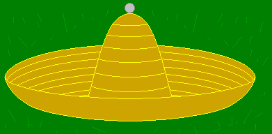
If you look down from above, the view will have perfect rotational symmetry – it won’t matter how you rotate the view, it will look the same:

Now let go of the marble. It will roll down the side of the hat into the rim:

The view will no longer have perfect rotational symmetry – the marble will mark out a particular direction:

The starting point of the marble represents a position of high potential energy. When the marble is released, this potential energy is converted into kinetic energy and the ball rolls down the side of the hat. The equations of motion which govern the way it moves are perfectly symmetric – they do not change under a rotation. However, when the marble finally comes to rest, the symmetry has been broken; this is a state of minimum energy.

This is exactly what happens in Salam and Weinberg’s theory. In fact, there is a potential energy term in the Lagrangian called a “Mexican Hat” potential. It’s called this because if you plot the way the potential energy varies with the values of the Higgs fields, the shape you get is, roughly speaking, the shape of a sombrero. In this theory, the interactions between the fields in a high-energy state are associated with a set of symmetries. The equations of motion are preserved under all of these symmetries. When the system is allowed to settle down into a low energy state, all but one of these symmetries are broken. (The Higgs fields are a set of scalar fields which have the original full symmetry.)

The symmetry which remains at low energies is the one associated with electromagnetism. The broken symmetries are associated with the weak interaction. This gives the weak interaction some very strange properties. It is mediated by particles with very large masses, known as W and Z particles. These high masses meant that they weren’t observed until 1983, when they were created in a particle accelerator. Until then, only their effects on other matter had been observed, in which they change particle identities and are responsible for nuclear beta decay and a particular type of supernova.

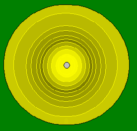
It’s also possible to use an analogy to demonstrate this idea of some of the symmetries being broken, while others remain unbroken at low energies. Imagine a transparent hollow sphere, with a bead at the very centre:

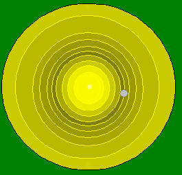
This system has perfect rotational symmetry in three dimensions. Imagine there is a force which attracts the bead to the surface of the sphere, which grows in strength the closer the bead gets to the surface. Once the bead is released, it will start to move towards the sphere’s surface, increasing in pace until it hits the surface, where it comes to rest:

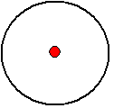
This marks out a “preferred direction”. We can choose an axis which runs through the bead and the centre of the sphere:

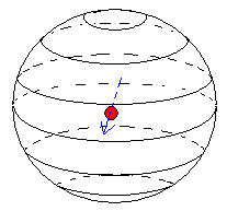
Rotating the sphere about this axis leaves it unchanged:

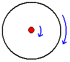
But rotating through any other axis will change the view. Thus we have broken the symmetry. The equations describing the system have three-dimensional rotational symmetry, as described above. However, the final state is only symmetric under rotations about one particular axis, that is, a group of rotations in two dimensions. All the other symmetries have been broken.

I have written notes on this particular symmetry breaking scheme and how it applies to field theory:

Non-linearly realised O(3) symmetries »

Spontaneous compactification

The only interactions in Kaluza and Klein’s theory (see page “Warping”) were gravity and electromagnetism. The symmetries of the theory were the symmetries of those interactions. Over the following decades there were a handful of papers looking at extending these ideas to include other symmetry groups. This required more than one additional dimension. These extra dimensions would be “compact”, that is, “rolled up” in some way.

However, one of the greatest shortcomings of all of these papers was that there was no explanation of why the extra dimensions should be compact. A possible explanation was provided with the concept of “spontaneous compactification” in the late 1970s and early 1980s. The basic idea was that symmetry breaking could cause the extra dimensions to become compact.

The first papers achieved this by making use of a set of scalar fields with a “Mexican hat” potential or similar. These are essentially Higgs fields which don’t just cause symmetry breaking but also cause the additional dimensions to become compact.

Some later papers avoided using scalar fields. In these later papers, there was a field associated with the non-gravitational interactions, such as the electromagnetic field or the “gluon” field of the strong interaction, included in the Lagrangian. This field acted as a matter distribution and caused the higher-dimensional spacetime to curve. It curved in such a way as to leave the additional dimensions compactified. It was then shown that in some cases, these new theories were equivalent to the ones with scalar fields.

But with either type of spontaneous compactification, the additional fields do not have the full symmetries of the higher-dimensional spacetime.

In recent years, this has been the focus of my research. I have developed a theory which resolves this problem. It is described in this preprint:

Covariant Compactification: a Radical Revision of Kaluza-Klein Unification

This theory has evolved quite a bit since I started developing it. Originally, I assumed that the theory would be governed by a Lagrangian constructed from fields. Under changes of coordinate system on the higher-dimensional spacetime, the fields would transform in the appropriate way – for example, scalar fields would not change, while the components of a vector field would mix up in the right way for a higher-dimensional vector. In this sense, every set of fields in the Lagrangian would transform according to the full symmetries of the higher-dimensional spacetime – and they would have no other transformation properties; there would be no other group of transformations acting on them. There would then be a symmetry-breaking process which would break these symmetries and cause the extra dimensions to compactify. The unbroken symmetries – those of the resulting spacetime – would include those underlying general relativity.

What I found is that rather than using a set of scalar Higgs fields, the theory needed to include a vector field. In the last few years, I’ve identified this vector field as the field of vectors tangent to a set (technically a “bundle” or “congruence”) of paths through spacetime. The field equation can be obtained from a Lagrangian, which is constructed entirely from this vector field and its covariant derivatives – quantities which describe how the vector varies between tangent spaces. The field equation is the simplest possible extention of Poisson’s equation which a) is valid in any frame of reference/coordinate system and b) describes gravity as a curvature of spacetime.

Furthermore, it turns out that we don’t actually need a Lagrangian. Any vector field defined in this way turns out to satisfy a field equation. Now, bodies and light rays in general relativity follow a particular kind of path called a geodesic. If the paths used to construct the crucial vector field are geodesics, the field equation simplifies to that which can be obtained from a Lagrangian. Thus we don’t need the machinery of the Lagrangian formulation: the same result can be obtained without it, simply by focusing on geodesics and their tangents.

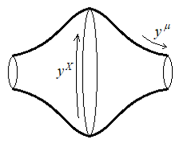
There exist solutions of these field equations in which the symmetries of the higher-dimensional tangent space break and the tangent spaces themselves separate. One can define scalar fields constructed from powers of the vector field’s covariant derivatives. These determine the way the symmetries break, which allows us to classify such solutions. For example, say we start with a six-dimensional spacetime. It is possible to choose relations between the powers of the covariant derivative such that the six-dimensional tangent space breaks into a four-dimensional one and a two-dimensional one. The metric splits, or “decomposes”, into separate metrics for the four-dimensional and two-dimensional tangent spaces. Similarly, vector fields then split into four-dimensional vector fields and two-dimensional ones.

I have been able to show that there are solutions of the field equation in which the universe has a tube-like geometric structure, in which the extra dimensions are compact. For example, with six dimensions, the extra two dimensions have the same shape as the surface of a sphere. The curvature of such a compact space may be constant across our four-dimensional spacetime (for example, for a circle or sphere, the radius may be constant), or it may vary, as indicated in the diagram below:

These geometric structures, their symmetries and the scalar quantities which classify them are explored in this paper:

Product manifolds as realisations of general linear symmetries

Preprint of an article published in International Journal of Geometric Methods in Modern Physics, 2021 https://doi.org/10.1142/S0219887822400060 © World Scientific Publishing Company

It has also turned out that there is no physical process which breaks the higher-dimensional symmetry. It’s just that the higher-dimensional symmetry is not explicit when you use a sensible set of coordinates on the tube-like structure. In the most general coordinates, which aren’t really sensible ones to use, the higher-dimensional symmetry becomes apparent.

You can, however, explore this symmetry by considering a mathematical limit: increase the radius of the compact space – the sphere or similar subspace. If you keep increasing it, the curvature of the surface of the tube keeps reducing. Eventually, if you increase the radius to infinity (and you reduce the curvature of four-dimensional spacetime to zero), you end up with a spacetime which is flat in all directions. In this limit, all the fields have the full higher-dimensional transformation properties, even in sensible coordinates. Thus it’s not true to say that in this theory, “symmetry is broken at low energies”. Instead symmetry is broken when the spacetime curvature is non-zero.

When the curvature of the compact space is constant over our four-dimensional spacetime, any object travelling in our familiar four-dimensional spacetime travels purely in that spacetime. Similarly, a path in the extra compact dimensions stays in those dimensions. But when the curvature of the compact space varies over our four-dimensional spacetime, other paths are possible which don’t stay entirely within these subspaces. This is because of the presence of extra components in the connection. These describe non-gravitational interactions. So when you see a science fiction film in which adventurers travel into other dimensions, consider this: every non-gravitational interaction may represent spacetime curving in such a way as to allow paths into additional dimensions.

Indeed, I did wonder if every particle we are made of, every electron, proton and neutron, may be an interdimensional traveller. However, I’m now exploring whether it’s possible that these may be patterns formed by the vector field. If this turns out to be the case, then we are all ultimately composed of fluctuations and wrinkles in spacetime.